Excel2010中制作两个纵坐标的操作方法

在用excel图表表达一组数据时，我们经常遇到几组有关联的数据，我们怎么在一个图表中表达他们呢?当然可以在一个图表中设置两个纵坐标，形成如下图的形式。今天，小编就教大家在Excel2010中制作两个纵坐标的操作方法。

Excel2010中制作两个纵坐标的操作步骤如下：

1、当然是有需要做成图表的数据。

2、点击菜单栏上的插入，在下拉列表中选在图表。

3、选择图表类型折线图，再选择数据点折线图作为子图类型。(这里根据个人喜好或者需要选择，不一定非要选择这种图表类型)

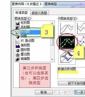
4、选择好图表类型，直接点完成(你也可以按照他的向导一步一步点下一步)。出现一个空白的图表，在空白的图表上右键，选择源数据。

5、在出现的源数据对话框中，选择系列——添加——输入系列名称(收入)——选择数据——在数据上框选---回车。

6、再点添加——输入系列名称(支出)——选择数据——回车。如图所示。

7、在生成的图表上的支出线上右键选择数据系列格式。

8、依次选择，坐标轴——次坐标轴——最后点击确定。

9、到这里基本完成了，为了更好分辨哪个坐标表示的哪一部分，可以在图表空白区域右键选择图表选项，在标题一栏下，分别填入两个坐标对应的名称。具体操作如图。

自定义类型一个图表中两个纵坐标。

1、基本步骤与上面相同，这里重点说不同点。选择图表类型时，选择——自定义类型——两轴折线图——点击下一步——添加系列——选择数据——回车——添加系列——选择数据——回车——确定。相同部分就不上图了。

2、这个方法比上面少了一步就是在数据线上右键选择次坐标轴。自定义类型少了这一步应该说是更简单了，大家可以尝试一下，其他图表类型相同，教程中用的是excel2003，用excel2007和2010的操作基本相同，不再赘述，赶快试一下吧。

注意事项：

自定义类型不用右键选择数据系列格式再选择次坐标轴了。直接选择好数据点确定就ok了!