怎么使用Excel2013中条件格式

条件格式，在Excel表格中十分有用，今天小编要讲的就是条件格式中一个简单的功能--突出显示单元格规则，让特殊的值以特殊颜色显示出来，便于区分，下面小编就不多废话，正如主题吧。

Excel2013中条件格式的使用步骤：

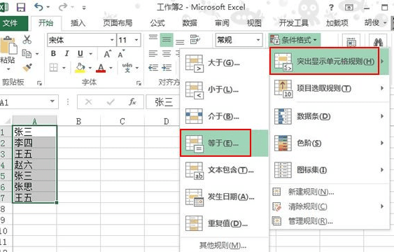
①选中表格数据，单击菜单栏--开始--条件格式--突出显示单元格规则--等于。

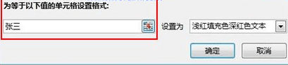
②在等于选项框中输入张三，颜色选为浅红填充色。

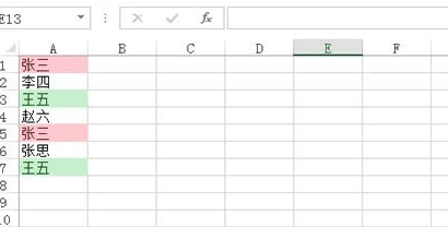
③此时数据为张三的单元格被浅红色填充了。

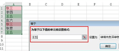
④再来对数据为王五的进行绿色填充，最后的效果大家看下面的图。